VFGEN § LSODA

LSODA Fortran 77 ODE Solver

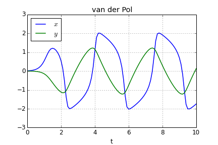
The ODEPACK suite includes the ordinary differential equation solvers LSODE, LSODA, and LSODAR. LSODE was written by A. Hindmarsh; LSODA and LSODAR were written by A. Hindmarsh and L. Petzold.

The VFGEN LSODA Command

A Fortran 77 file that can be used with LSODE, LSODA, or LSODAR is created by the command

$ vfgen lsoda vector_field_file.vf

This command creates the Fortran file [name]_rhs.f, where [name] is the name of the vector field given in the vector field file. The file contains the following subroutines:

[name]_rhs The vector field function (right hand side)
[name]_jac The Jacobian of the vector field

Options

func	If the option func=yes is given, VFGEN creates a subroutine that computes the values of any Functions that were defined in the vector field file. The subroutine is designed to be used with the rootfinding capability of the LSODAR solver. Default: func=no
parstyle	There are two methods for passing parameters to the vector field and Jacobian functions: include them in the array that holds the state variables, or put them in a named common block. The parstyle option allows you to choose which method to use. If the option parstyle=common is given, the parameters will be put in a common block with the name [name]_parameters, where [name] is the name of the vector field. If the option parstyle=after is given, the parameters are included in the same vector as the state variables, beginning just after the last state variable. Default: parstyle=after
demo	If the option demo=yes is given, the file [name]_demo.f is also created. This program provides a sample driver for the LSODA subroutine. The initial conditions and parameter values are the default values defined in the vector field file. Default: demo=no

Notes

Two non-standard features of the compiler are used: the Fortran code is written in lower case, and the underscore is used in variable names (e.g. y_). The underscores are an easy way to avoid conflicts with variable names that are taken from the vector field file. (If you need code without underscores, let me know.)

Example 1

Here is a sample vector field file: vanderpol.vf.
The files created by

$ vfgen lsoda:demo=yes vanderpol.vf

are

In a Linux (or similar) system, the following commands will compile and run vanderpol_demo.f using the gfortran compiler.

$ gfortran -c -w opkdmain.f opkda1.f opkda2.f
$ gfortran -c vanderpol_rhs.f
$ gfortran -c vanderpol_demo.f
$ gfortran vanderpol_demo.o vanderpol_rhs.o opkdmain.o opkda1.o opkda2.o -o vanderpol_demo
$ ./vanderpol_demo > vdp.dat

The last command runs the program and sends the output to vdp.dat. Here is a plot of the data:

Example 2

The Rossler system is

x '	=	-(y+z)
y '	=	x + ay
z '	=	b + (x-c)z

A vector field file for this system is rossler.vf. This file defines a Function which is simply the y value. This function will be used with the root-finding capability of the LSODAR function to find the points where trajectories cross the plane y = 0.

We create a Fortran implementation of the vector field with the command

$ vfgen lsoda:func=yes rossler.vf

This creates the file rossler_rhs.f.

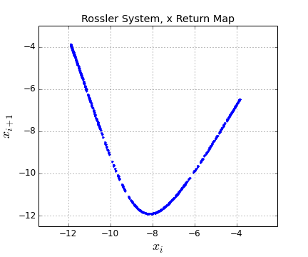
The program rossler_pmap.f uses the root-finding capability of LSODAR to compute the points where a trajectory crosses the plane y = 0 (and x < 0). The resulting x return map is plotted in the following figure.